I and my study group took a course on Regressors and I felt I’d like to write an article on the basics of the Support Vector Machines but then I thought why not give a brief intro to Linear regressors first and here we are. In this article, I’d be writing about all I know about Linear Regressors, the intuition behind them and their applicability. I hope you’d follow along and learn a few things.

Linear Regressors are a type of supervised machine learning in which a model tries to match a relationship (a linear type) between individual features in a feature set or a feature vector to the target variable on a straight line or hyperplane. Mathematically, it is usually represented as:

The x representing the values of each independent variable in our data instance, b0 corresponding to the intercept of the linear relationship between the independent variables and the target variable on the y-axis and b1 representing the regression coefficient or weight. In the case of a linear regression, a typical regression model tries to predicts the optimum combination of weights b1, b2…, bn given a constant coefficient b0 that leads to a target value y, reproduceable across all data instances in our dataset. The predicted weights would usually determine the relationship of the independent variables with our target variable.

There are several types of linear regression models as well as several techniques of implementing them. The python scikit-learn package affords us the opportunity to work with some of these methods of implementing linear regression models on our dataset and I would talk a little bit about some of them as we move on.

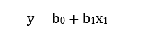
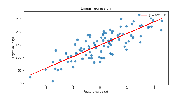
Simple Linear Regression: In this case, as explained above, the linear regression aims at illustrating the relationship between a single input feature, x, and a desired output, y, on a straight line using the simple straight-line equation;

In the linear regression equation, the values b0 and b1 is known as the intercept and slope respectively.

Multi Linear Regressions: The multi-linear regression is an expansion of the simple linear regression where by we have two or more features set having relative contributions or effect on the prediction of the desired output. The linear regression we saw earlier now looks something like;

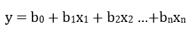where n would indicate the number of features to be considered

Polynomial Regression: Its scikit-learn implementation is usually used when extra features due to interaction between data features needs to be generated. Its implementation in any data science project could lead to an improved model. It is good to keep in mind that its interpretability decreases with increasing degrees of the polynomial as the model becomes more complex.

from sklearn.linear_model import Ridge 
# There are infact any more models we can find in the sklearn.linear_model module
from sklearn.datasets import make_regression
from sklearn.model_selection import train_test_split
from sklearn.preprocessing import PolynomialFeatures

X_R1, y_R1 = make_regression(n_samples= 100, n_features=3,
n_informative= 2, bias = 150.0,
noise = 30, random_state= 0)

X_train, X_test,y_train, y_test =  train_test_split(X_R1, y_R1, random_state = 0)

print('Shape of train data features before transforming: ', X_train.shape)

poly = PolynomialFeatures(interaction_only= True, include_bias= False)
X_train_poly = poly.fit_transform(X_train)
X_test_poly = poly.transform(X_test)

print('Shape of train data features after transformation', X_train_poly.shape)

The output is given as:

Shape of train data features before transforming:  (75, 3)
Shape of train data features after transformation (75, 6)

# Nicee, we have created twice as much features

Some methods of implementing the multilinear regression model provided by scikit-learn includes:

• Lasso Regression: performs a sort of feature selection by limiting the weight of ‘irrelevant’ features to the values of zero so they do not have a contribution to the prediction of our target output.

• Ridge Regression: In this type of linear regression, the optimal combination of weight leading to the least value of the mean of squared errors of each data instance in our dataset is determined by restricting the weight parameters to smaller values with a reduced variance.

Other implementation of the Linear regression model provided by the scikit-learn package include Logistic Regression and the Linear Support Vector Machines which we would cover in some other article

linreg = Ridge().fit(X_train, y_train)

print("\nAccessing the Regression model parameters:")
print('\nLinear model coeff (w): {}'
     .format(linreg.coef_))
print("Linear Model intercept (b): {:.3f}"
     .format(linreg.intercept_))

print("\nChecking Score Metrics of the fitted Linear Regression Model:")

print('\nR-squarers score (training): {:.3f}'
     .format(linreg.score(X_train, y_train)))
print('R-squared score (test): {:.3f}'
     .format(linreg.score(X_test, y_test)))

We have our output as:

Accessing the Regression model parameters:

Linear model coeff (w): [61.55 40.53  2.87]
Linear Model intercept (b): 141.813

Checking Score Metrics of the fitted Linear Regression Model:

R-squared score (training): 0.889
R-squared score (test): 0.802

In terms of applicability, the linear regression is sometimes preferred ahead of complex ensembles models in industrial applications due to its ease in interpretation in cases where a firm might want to determine what features are driving a desired output and what features are likely to not have any effect. You might want to consider using Linear regression models if you want to use models that;

• Do not require too much of parameter tuning and are easy to train
• Predict results quite fast
• Perform well on sparse data or data with a lot of zero values
• Scale well to large dataset

Cover Photo from Openbootcamps